Spring Mass System Simulator
Today we’re gonna take a look at solving the equations of motion for a spring mass system. Now, you may be asking: solving a what? Well, imagine you wanted to simulate the motion of a piece of elastic fabric hung up on a wall, or the motion of atoms in molecules (and believe me, sometimes you $do$ want to). Such systems can be described by spring mass systems. These are systems that contain multiple bodies with mass that are connected by springs. Of course, the connections can be arbitrary and the “stiffness” of the springs (the spring constant) can be different for every spring. There are also one or more fixtures we can tether the masses on, so they won’t just enter free fall.
You can find the complete code in my GitHub repository at https://github.com/sdomoszlai13/spring-mass-system-simulator.
The program we’ll get to know runs a simulation of a system of fixtures, masses, and springs in two dimensions. Fixtures and masses can be set up with initial coordinates and initial velocities (not for fixtures, of course). After setting the desired temporal length and the number of time steps, the simulation is run and a plot is created with the fixtures, masses, and the masses’ trajectories so we can see which way they went. There’s also an option to save the trajectories to a file.
Physical Background
Consider a mass $m$ attached to a spring with a spring constant $k$ moving in 1D. Then, the equation of motion of the mass is:
\[m\ddot{x}(t) = -kx + mg,\]where $x(t)$ is the position of the mass and $g$ is the gravitational acceleration. If two masses are coupled in series, the system can be described by a set of equations (omitting time dependence notation for simplicity):
\[m_1\ddot{x_1} = -k_1x_1 + k_2(x_2-x_1) + m_1g,\] \[m_2\ddot{x_2} = k_2(x_2-x_1) + m_2g.\]If we allow the masses to move in 2D, the equations become
\[m_1\ddot{\vec{x_1}} = -k_1(||\vec{x_1}|| - l_1)\frac{\vec{x_1}}{||\vec{x_1}||} + k_2(||\vec{x_2} - \vec{x_1}|| - l_2)\frac{\vec{x_2} - \vec{x_1}}{||\vec{x_2} - \vec{x_1}||} + m_1\vec{g},\] \[m_2\ddot{\vec{x_2}} = -k_2(||\vec{x_2} - \vec{x_1}|| - l_2)\frac{\vec{x_2} - \vec{x_1}}{||\vec{x_2} - \vec{x_1}||} + m_2\vec{g}.\]A general system of springs and masses can be described by a similar set of equations. By solving the equations for $x(t)$, we can determine the trajectories of the masses. In principle, these equations can be solved analytically. However, that’s more of a maths problem than a software development problem. For the sake of simplicity, we’re gonna solve the equations numerically with the help of the (forward) Euler method. This is a quite simple method to solve differential equations and works as follows.
Let’s suppose we know the position $x(t)$ and the velocity $v(t)$ of a mass at the time $t$, as well as the force $F(t)$ acting on it. A small time $\Delta t$ later, at the time $t’ = t + \Delta t$, we can say that approximately
\[x(t') = x(t) + v(t)\Delta t,\] \[v(t') = v(t) + a(t)\Delta t = v(t) + \frac{F(t)}{m}\Delta t,\] \[F(t') = \sum_{j} F_{spring_j} + mg.\]To make use of this algorithm, we have to divide our simulation time into $n$ discrete time steps which a time difference of $\Delta t$. Then, for every time step, the new values of $x(t)$, $v(t)$, and $F(t)$ are calculated. The set of the values of $x(t)$ is the trajectory of the mass. These values can be stored in array and be plotted. This algorithm is implemented for an arbitrary number of masses moving in 2D by this program.
Software
The simulation is implemented in Python, as speed is not critical and there are great libraries available for numerical simulations in Python (NumPy, SciPy etc.), and MatPlotLib makes nice and easy plotting possible. An object-oriented approach was chosen for the simulation, as the the problem can be well described with an objects-centered approach. Fixtures, masses, springs, and even whole spring mass systems are all user-defined types in the program.
The program is devided in three files:
- main.py: contains everything needed to run a simulation
- user_input.py: contains functions for nice-and-easy user input to setup a simulation
- test.py: contains pre-built spring mass systems for testing purposes.
The main.py file contains the classes for the fixtures, masses, springs etc. The fixtures can be implemented relatively straight forward.
class Fixture:
    """
    Initialize a fixture.
    Attributes:
    -pos: position
    -attached: attached objects (mass(es) and/or spring(s))
    """

    def __init__(self, x, y):
        self.pos = [x, y]
        self.attached = [] # List format: [mass/fixture connected to this fixture,
                           #               spring constant of connecting spring,
                           #               rest length of connecting spring]
For the masses, there are some important things to consider. The initial position and initial velocity is are passed component-wise. The constructor creates the corresponding vectors and initializes them accordingly. The Mass class has a trajectory attribute. This way, every mass object has its trajectory “attached” to it - just as in reality. After careful considerations, the author concluded it would be best to make masses “know” which fixtures and/or objects are connected to them. This comes in handy later: it makes a well-readable calculation of the force acting on the masses possible.
class Mass:
    """
    Initialize a mass.
    Attributes:
    -m: mass
    -pos: position
    -v: velocity
    -f: acting force
    -attached: attached objects (mass(es) and/or spring(s))
    -trajectory: trajectory
    """

    def __init__(self, m, x0, y0, vx0, vy0):
        self.m = m
        self.pos = [x0, y0]
        self.v = [vx0, vy0]
        self.f = []
        self.attached = [] # List format: [mass/fixture connected to this fixture,
                           #               spring constant of connecting spring,
                           #               rest length of connecting spring]
        self.trajectory = [self.pos]
The Spring object is implemented as shown below.
class Spring:
    """
    Initialize a spring that connects a fixture and a mass, or two masses.
    Attributes:
    -l0: rest length
    -k: spring constant
    -conn: objects that the spring connects (list of mass(es) and/or fixture(s))

    Connecting mass(es) and/or fixture(s) must be provided as a list
    """

    def __init__(self, l0, k, conn):
        self.l0 = l0
        self.k = k
        self.conn = conn

        # Attach spring to second element (fixture/mass)
        self.conn[0].attached.append([conn[1], self.k, self.l0])
        self.conn[1].attached.append([conn[0], self.k, self.l0])
The Spring objects “know” (through an attribute) which fixtures and/or masses they connect. It’s worth noting that there’s no length attribute; the current length isn’t stored with the spring as it’s just needed for the force calculations. Thus, the spring lengths are calculated for every time step by calculating the distance between connected objects and used only to update the force values.
The SpringMassSystem class is implemented as shown below.
class SpringMassSystem:
    """
    Initialize the spring mass system.
    Attributes with similar names as in Mass and Fixture class
    are defined identical.
    Additional attributes:
    -time: length of time interval to be simulated
    -timesteps: number of intervals time is to be divided into
    -g: gravitational acceleration
    -save: control of function save() that saves trajectories in a file
    Fixtures, masses, and springs must be provided as lists
    """

    def __init__(self, fixtures, masses, springs, time = 1, timesteps = 100, save = False, g = 9.81):
        self.fixtures = fixtures
        self.masses = masses
        self.springs = springs
        self.g = -g
        self.timesteps = timesteps
        self.time = time
        self.delta_t = time / timesteps
        self.trajectories = []
        self.save_csv = save
        self.E_i = 0
        self.E_f = 0

        for m in self.masses:
            m.f = [0, m.m * self.g]
A Spring Mass System object has attributes that store the gravitational acceleration in the system, the number of time steps, the fixtures, masses, and springs etc.
And now for the fun part: doing the calculations. The function below calculates the relevant physical quantities (positions, velocities, forces) for the next time step.
def update(self):
    """
    Update positions and velocities of the masses, and
    the force acting on them
    """

    # Update forces
    for m in self.masses:
        m.f = [0, 0]
        for elem in m.attached: # elem = [other_mass_or_fixture, spring_constant, rest_length]
            m.f[0] += -elem[1] * (np.linalg.norm(np.array(elem[0].pos) - np.array(m.pos)) - elem[2]) * ((np.array(m.pos[0]) - np.array(elem[0].pos[0])) / (np.linalg.norm(np.array(elem[0].pos) - np.array(m.pos))))
            m.f[1] += -elem[1] * (np.linalg.norm(np.array(elem[0].pos) - np.array(m.pos)) - elem[2]) * ((np.array(m.pos[1]) - np.array(elem[0].pos[1])) / (np.linalg.norm(np.array(elem[0].pos) - np.array(m.pos)))) + m.m * self.g

    # Update positions
    for m in self.masses:
        m.pos[0] += m.v[0] * self.delta_t
        m.pos[1] += m.v[1] * self.delta_t
        m.trajectory.append(m.pos[:]) # Deep copy of pos
        # print(f"Added to trajectory: {m.pos}")

    # Update velocities
    for m in self.masses:
        m.v[0] += m.f[0] / m.m * self.delta_t
        m.v[1] += m.f[1] / m.m * self.delta_t
The calculations implemented are done based on the equations shown earlier (see section Physical Background). The advantage of the object-oriented approach really stand out here: as the update function is a member function of the SpringMassSystem class which “knows” of every fixture, mass, and spring, no function arguments are needed for the update function. Every relevant physical quantity is an attribute of the object (the same goes later for plotting). The NumPy library is used to calculate the vector norms. Note the importance of the deep copy when updating mass positions. This is a crucial step; otherwise, the trajectory won’t be updated properly.
Another member function of the SpringMassSystem class is the energy function. It’s used to calculate the total energy of a spring mass system at a given point in time. Doing these calculations at least at the beginning and the end of a simulation, the plausibility of the calculated trajectories can be checked.
def energy(self, t):
    """
    Calculate total energy of the system at a given point in time
    """

    E = 0

    # Calculate energy of masses
    for m in self.masses:
        E += m.m * m.trajectory[t][1] * self.g + m.m * (m.v[0] ** 2 + m.v[1] ** 2) / 2

    # Calculate energy of springs
    for s in self.springs:
        E += s[0].k * (np.linalg.norm(np.array(s[0].conn[0].pos) - np.array(s[0].conn[1].pos)) - s[0].l0)

    return E
There are also functions to save and plot trajectories. There’s nothing special about them and therefore, they won’t be discussed here.
Last but not least, there’s the run function. This function is called after the setup of the spring mass system is finished. It runs the simulation and plots trajectories. If wished, it also saves trajectories to a .txt file.
def run(self):
    """Run the simulation"""

    # Create time steps
    self.times = np.linspace(0, 1, self.timesteps)

    # Calculate initial energy of the system
    self.E_i = self.energy(0)

    # Update forces, positions and velocities. Create m.trajectory array for each m
    for t in self.times:
        self.update()

    # Save trajectories of all masses in a single array (trajectories).
    # One element of the array contains the coordinates of all masses at a given point in time

    # self.trajectories = [self.timesteps, 2, len(self.masses)]
    self.trajectories = []

    for t in range(len(self.times)):
        x_coords = [m.trajectory[t][0] for m in self.masses]
        y_coords = [m.trajectory[t][1] for m in self.masses]
        self.trajectories.append([x_coords, y_coords])

    # Calculate final energy of the system
    self.E_f = self.energy(self.timesteps)

    # Check plausibility of results
    self.energyCheck()


    # Save to file if user wishes
    if self.save_csv == True:
        self.save()
        print(f"Saved trajectories to \"trajectories.txt\"")

    # Plot trajectories
    self.plot()
Examples
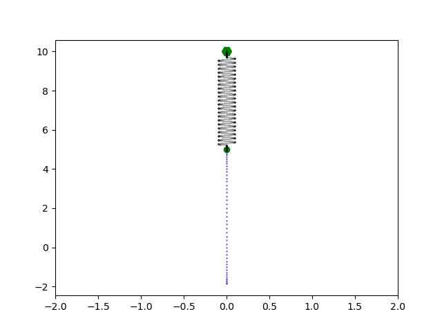
Let’s see what’s possible with a basic simulation tool like this. First, we try to simulate a vertically oscillating mass, also known as a harmonic oscillator.
Next, let’s look at a non-elastic pendulum.
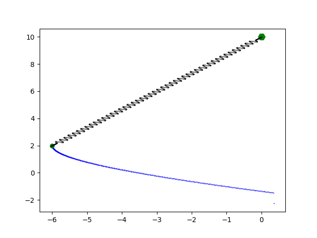
So far, so good. There’s nothing special going on here.
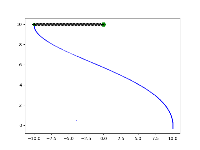
Now, let’s see what happens if we build an elastic pendulum.
Nice! Now we’re gonna take a look at a double pendulum.
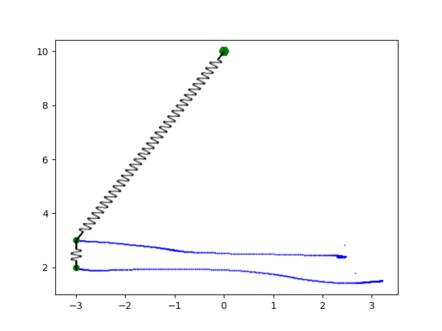
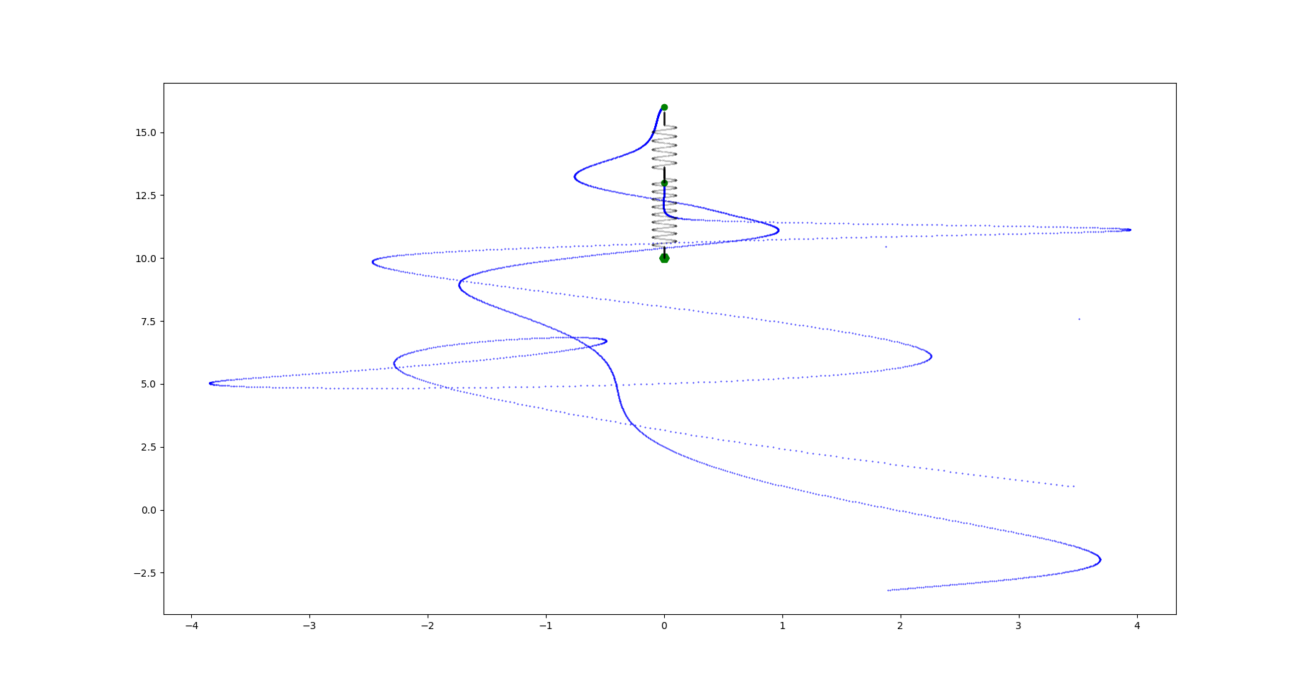
Double pendulums are actually quite fascinating because of their so-called chaotic behavior. This means that for slight variations in initial conditions, the resulting trajectories can be significantly different from one another. Such systems can be described with the help of chaos theory. But now, let’s create a bit more chaos, shall we? Here’s an elastic double pendulum.
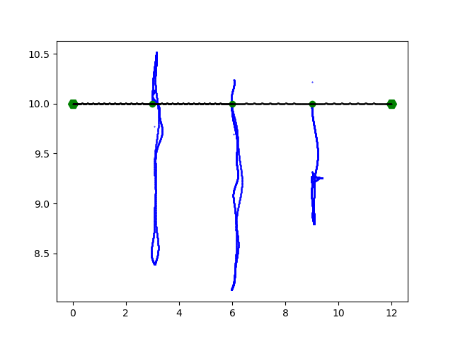
One more example: three masses tethered between two fixtures. The left mass has a low-value initial velocity in the vertical direction.
Isn’t it amazing what a basic algorithm for solving differential equations is capable of?
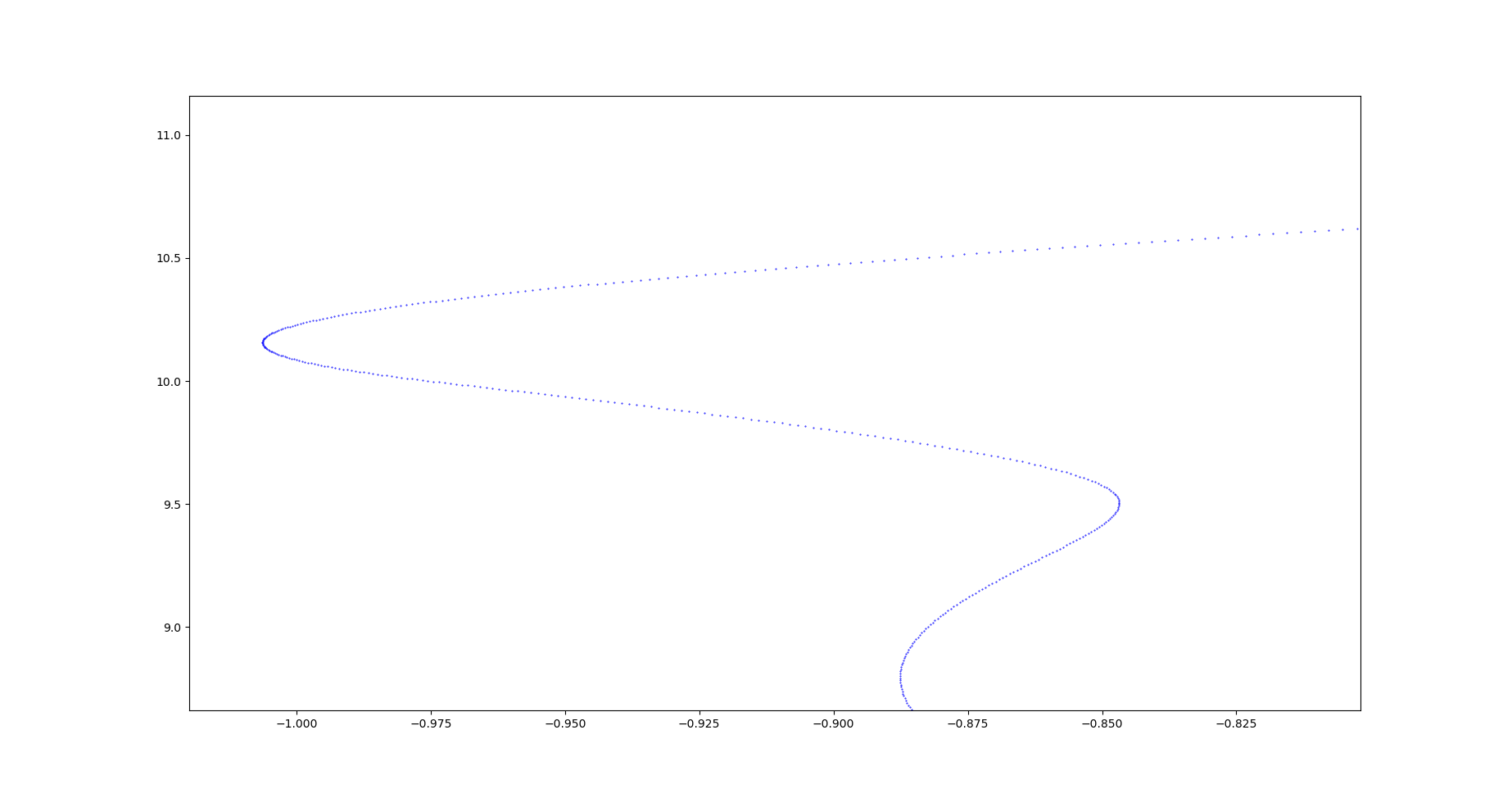
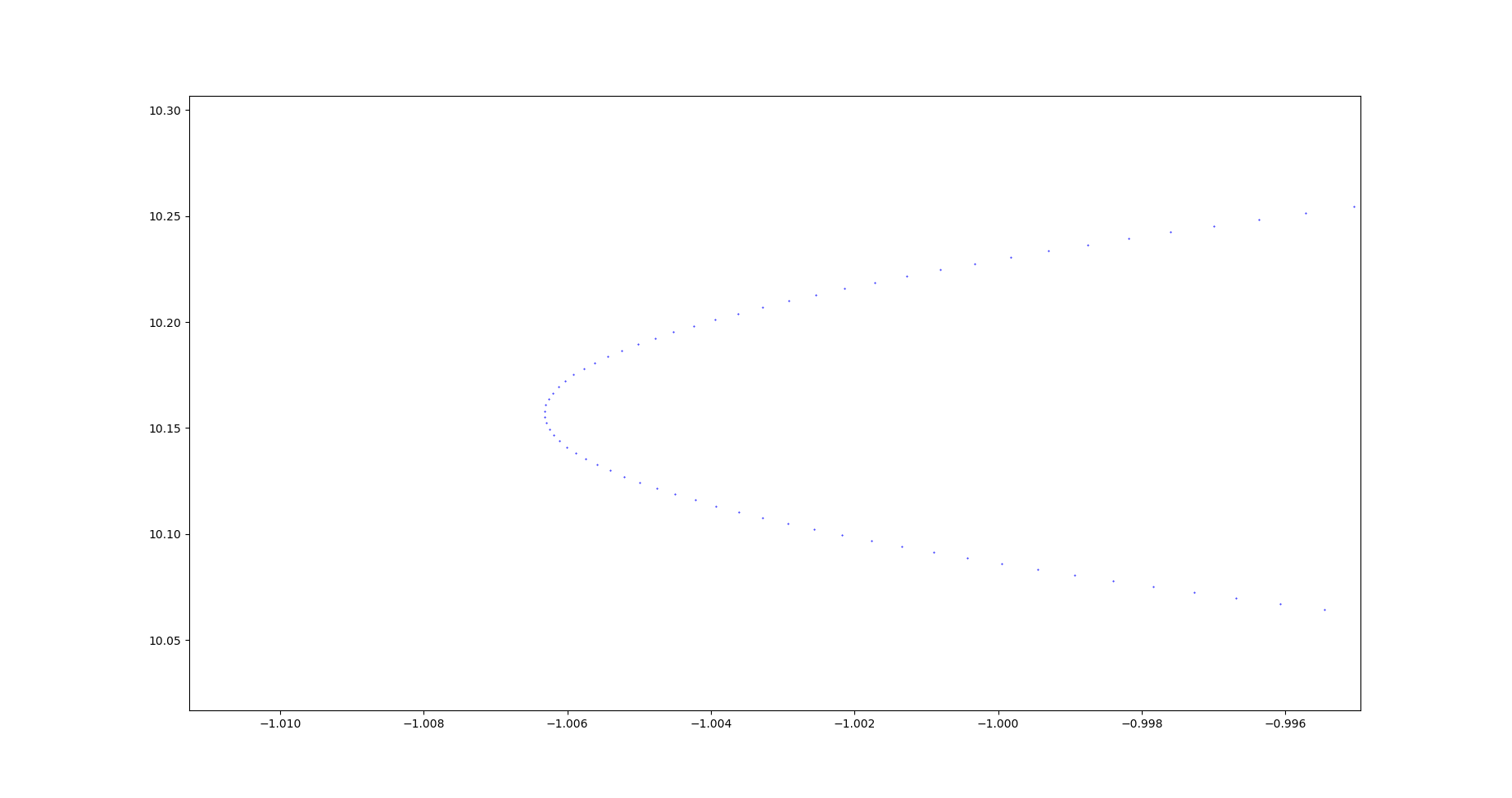
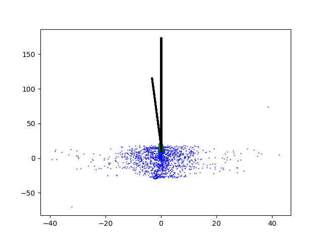
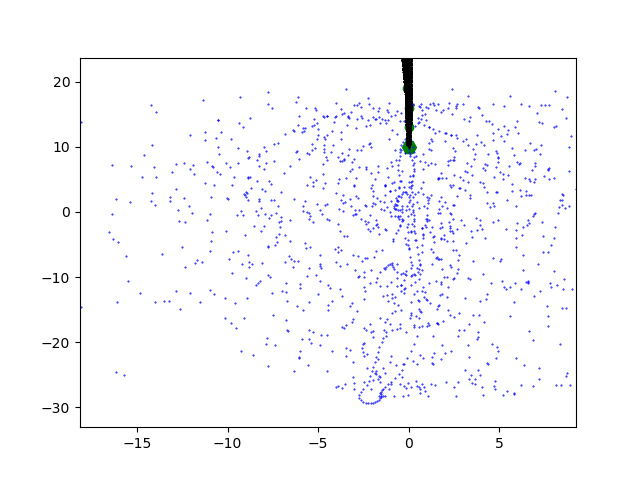
Of course, there are some pitfalls to avoid to get realistic results. Simulation time and the number of time steps is critical. There should be at least 1000 time steps for each second of simulation time, depending on expected velocities of the masses. Similarly, if the spring constant is increased, the number of time steps should also be increased. This is important because of higher velocities and accelerations. As the time steps are distributed equally on the time scale, calculated points on the trajectory are more spaced out if the velocity of a mass is higher. This can be seen in the image below.
If the number of time steps is too low, the solutions can diverge and plots as shown below appear.
Ever wondered what the the trajectory of a double pendulum would look like? Or even better: a triple pendulum? What about the placing of carbon atoms in a single-walled carbon nanotube? Now you can find out! Play around with this little simulation tool and see for yourself what’s possible in the world of frictionless spring mass systems!
Summary
The “brute force” approach of using the forward Euler method to solve the equations of motion for a spring mass systems is not the most efficient. However, it allows a swift introduction to the world of numerical simulations. If the simulation parameters are chosen wisely, one can get decent results, e.g. realistic trajectories of the masses of a triple pendulum or a chain of atoms.
You can find the complete code in my GitHub repository at https://github.com/sdomoszlai13/spring-mass-system-simulator.